Using the Weka Forecasting Plugin
Contents
1. Introduction
The Weka Forecasting plugin is a transformation step for PDI 4.x that is similar to the Weka Scoring Plugin. It can load or import a time series forecasting model created in Weka's time series analysis and forecasting environment and use it to generate a forecast for future time steps beyond the end of incoming historical data. This differs from the standard classification or regression scenario covered by the Weka Scoring plugin, where each incoming row receives a prediction (score) from the model, in that incoming rows provide a "window" over the recent history of the time series that the forecasting model then uses to initiate a closed-loop forecasting process to generate predictions for future time steps.
2 Requirements
The Weka Forecasting plugin requires PDI 4 or higher, Weka 3.7.3 or higher and the core time series forecasting library from the time series forecasting package. Both Weka and the time series forecasting core library are bundled with the plugin, so no further downloads are required.
3 Installation
The Weka Forecasting plugin is included with PDI enterprise edition. It can be found in Spoon's design palette under the "Data Mining" folder.
4 Using the Weka Forecasting Plugin
Once the forecasting plugin step is installed, and Spoon has been restarted, the Weka Forecasting step can be found in the "Transform" folder in the "Design" tab.
In this section we will demonstrate using the model developed on the Australian wine data in Section 3.1.1 of Time Series Analysis and Forecasting with Weka. This forecaster modeled monthly sales of the "Fortified" and "Dry-white" series. The following simple transformation loads the wine data and passes it to the Weka Forecasting step. The Weka Forecasting step uses the incoming data as historical "priming" data, that is, the data is used to populate the values of lagged variables and variables derived from the time stamp. These values are then input to the forecasting model and a forecast is produced for a user-defined number of steps beyond the end of the priming data. The step outputs the historical data followed by a number of new rows that contain the forecasted values.
Subsequent sections explain the configuration options for the step and the output that it produces in detail.
![]()
4.1 Loading or Importing a Forecasting Model
Conceptually, the UI for the Weka Forecasting step is set out in a similar fashion as the Weka Scoring plugin. The Model file tab allows a model to be loaded from the file system and configured for forecasting. 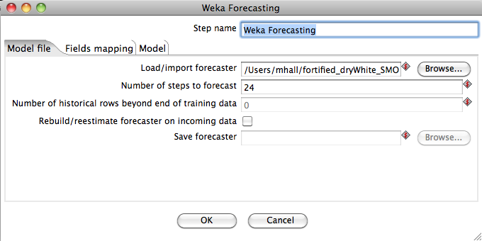
The Load/import forecaster field allows a serialized forecasting model to be loaded from a file. A path can be entered into the field directly, or the Browse button can be used to bring up a file browser dialog. If the field is left populated with a path then the forecasting model will be loaded from the file every time that the transformation is run. Alternatively, after importing a forecasting model (by pressing enter in the field after a path has been typed) or by using the Browse button, if the field is cleared and the OK button pressed then the model will be stored in the XML ".ktr" file or in the repository (if one is being used).
The Number of steps to forecast field allows the user to specify how many time steps into the future the model will produce predictions for. In this example we have entered "24" in order to get a monthly forecast out to 24 months beyond the end of the incoming priming data.
The Number of historical rows beyond end of training data field only becomes enabled when the step detects that the loaded forecasting model is using an artificial time stamp (see Section 3.1.2 of Time Series Analysis and Forecasting with Weka). In this case, the user can specify how many rows of the incoming priming data occur after the most recent row seen by the forecaster when it was trained - this enables the forecaster to synchronize the artificial time stamp value with the priming data.
The Rebuild/reestimate forecaster on incoming data check box allows the user to specify that the forecaster should be trained on the incoming data rather than primed. This allows the forecasting model to be brought up to date with the latest historical data. After training is complete, a forecast is generated as described above. Selecting this option enables the Save forecaster field. This field can be used to specify a file to which the updated forecasting model will be saved out to. Leaving the field blank tells the step not to save the updated forecasting model.
4.2 Checking Data Fields
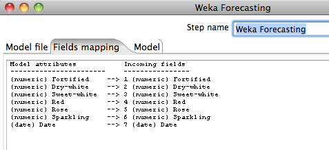
The Fields mapping tab allows the user to check how the step is mapping incoming transformation fields to those that the model saw in its training data. The step matches both field names and types - note that this is done between incoming Kettle fields and the original training data fields (before any internal transformations done by the forecasting model itself). Any training data fields that don't have counterpart in the incoming data are indicated by an entry labelled "missing". If there is a difference in type between a training field and an incoming field, then this will be indicated by the label "type-mismatch". In both cases, the forecaster will receive a missing value as input for the field in question for all incoming data rows. This will impact forecasting performance to a greater or lesser degree.
4.3 Checking the Model
The Model tab allows the user to check that model loaded is actually the one that he or she intents to use. This tab displays the textual description of the forecasting model in exactly the same way as it appears in the output of the time series forecasting environment. 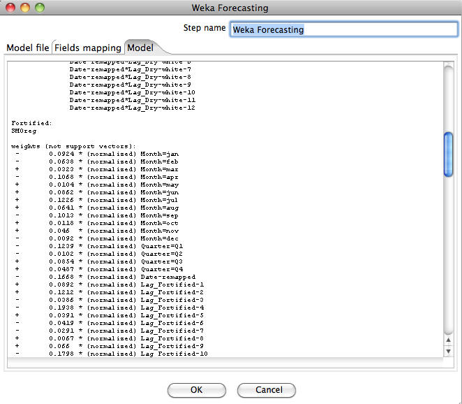
4.3 Output
The following screenshot shows a preview of the rows output by the Weka Forecasting plugin step for the Australian wine forecasting model. Historical rows are output first - values for all the types of wine are present in these rows. Forecasted values follow the historical rows. In the case of this model, the forecasted values for the "Fortified" and "Dry-white" types of wine occur in rows towards the end of the output (where the values for the other types of wine are missing). The values of the confidence bounds on these two types of wine are also present for these rows. Note that confidence bounds will only be output for future time steps that were defined when the model was trained. For example, if the user specified a forecast for 12 future time steps in the Basic configuration panel of the time series analysis and forecasting environment, and turned on the computation of confidence intervals, then confidence intervals will only be output for up to 12 time steps into the future. The user can request forecasts for more than 12 time steps but predictions beyond 12 steps into the future will not have confidence limits output. 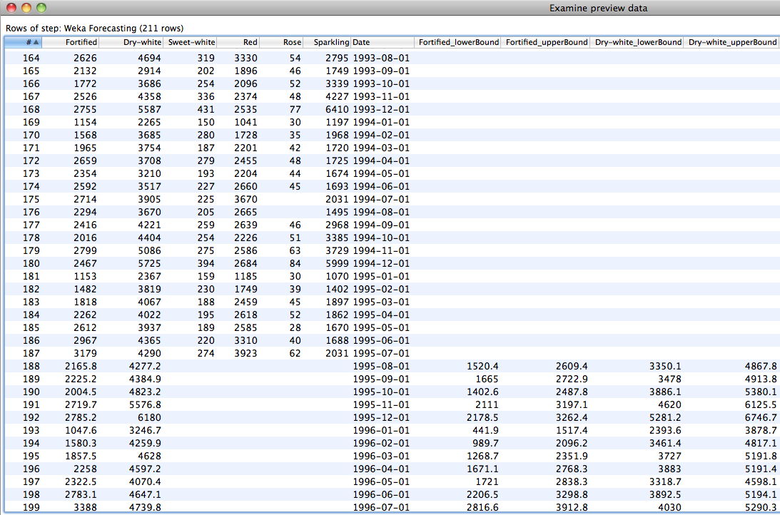
4.5 Using Overlay Data
The time series analysis and forecasting environment documentation (Section 3.2.4) explains how external "overlay" fields (sometimes called intervention data) can be incorporated into a forecasting model. If such data has been used to train a forecasting model used in the Weka Forecasting plugin step then this data must be supplied for the future time periods for which forecasted values are requested. This is accomplished by including rows in the incoming data stream for future time steps that contain values for the time stamp (if in use) and values for the overlay fields that the model is expecting. In this case, the number of these rows provided determines the number of forecasted values that will be produced, and the Number of steps to forecast field in the Model file tab is ignored.
IMPORTANT
In order for the step to be able to identify, in the incoming data stream, where historical priming/training data finishes and future overlay data begins, it is crucial that the values for the forecasted target field(s) are missing in the future overlay data.
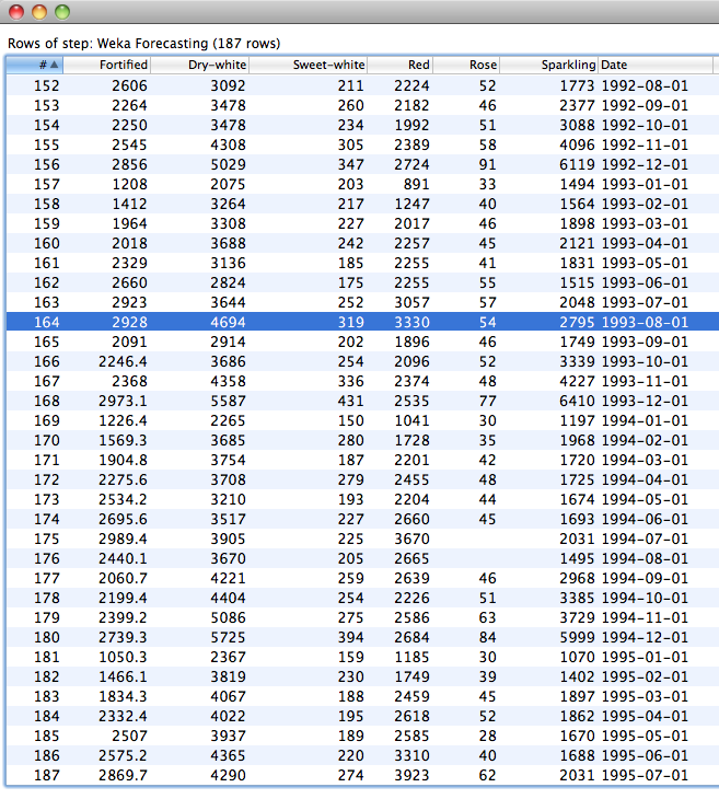
The following screeshot shows previewing an input data set that contains overlay data for future time steps to be forecasted. The data is the Australian wine data again. The model is predicting "Fortified" and expecting to use "Dry-white" and "Sweet-white" as overlay data.
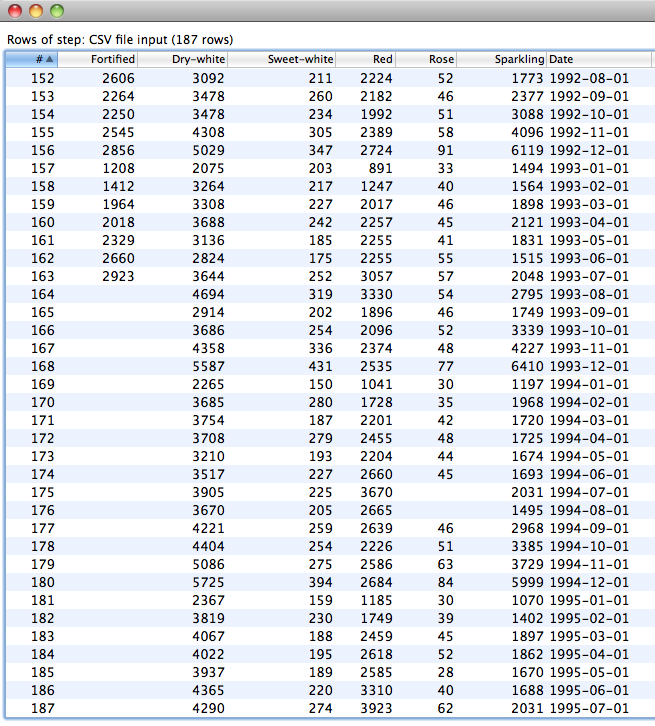
In this case we are treating the data from August 1993 onwards as "future" time steps to be predicted. It can be seen that values for "Fortified" (our single target in this case) are missing from this point onwards; whereas the values of "Dry-white" and "Sweet-white" (our "overlay" data) are present. Note that there are two missing values for "Rose" as well - these are truly missing in the original data, but have no affect on the model because Rose is neither a target or an input.
The following screenshot shows the output of the step on this data (no confidence intervals are being produced in this example). We can see that the forecaster has now filled in the values of "Fortified" for the future time steps in the overlay rows of the data.