Time Series Analysis and Forecasting with Weka
Contents
1 Introduction
Time series analysis is the process of using statistical techniques to model and explain a time-dependent series of data points. Time series forecasting is the process of using a model to generate predictions (forecasts) for future events based on known past events. Time series data has a natural temporal ordering - this differs from typical data mining/machine learning applications where each data point is an independent example of the concept to be learned, and the ordering of data points within a data set does not matter. Examples of time series applications include: capacity planning, inventory replenishment, sales forecasting and future staffing levels.
Weka (>= 3.7.3) now has a dedicated time series analysis environment that allows forecasting models to be developed, evaluated and visualized. This environment takes the form of a plugin tab in Weka's graphical "Explorer" user interface and can be installed via the package manager. Weka's time series framework takes a machine learning/data mining approach to modeling time series by transforming the data into a form that standard propositional learning algorithms can process. It does this by removing the temporal ordering of individual input examples by encoding the time dependency via additional input fields. These fields are sometimes referred to as "lagged" variables. Various other fields are also computed automatically to allow the algorithms to model trends and seasonality. After the data has been transformed, any of Weka's regression algorithms can be applied to learn a model. An obvious choice is to apply multiple linear regression, but any method capable of predicting a continuous target can be applied - including powerful non-linear methods such as support vector machines for regression and model trees (decision trees with linear regression functions at the leaves). This approach to time series analysis and forecasting is often more powerful and more flexible that classical statistical techniques such as ARMA and ARIMA.
The above mentioned "core" time series modeling environment is available as open-source free software in the CE version of Weka. The same functionality has also been wrapped in a Spoon Perspective plugin that allows users of Pentaho Data Integration (PDI) to work with time series analysis within the Spoon PDI GUI. There is also a plugin step for PDI that allows models that have been exported from the time series modeling environment to be loaded and used to make future forecasts as part of an ETL transformation. The perspective and step plugins for PDI are part of the enterprise edition.
2 Requirements
The Weka time series modeling environment requires Weka >= 3.7.3 and is provided as a package that can be installed via the package manager.
3 Using the Time Series Environment
Once installed via the package manager, the time series modeling environment can be found in a new tab in Weka's Explorer GUI. Data is brought into the environment in the normal manner by loading from a file, URL or database via the Preprocess panel of the Explorer. The environment has both basic and advanced configuration options. These are described in the following sections.
3.1 Basic Configuration
The basic configuration panel is shown in the screenshot below: 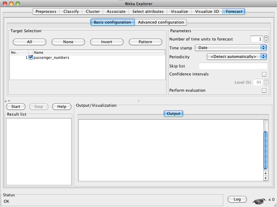
In this example, the sample data set "airline" (included in the package) has been loaded into the Explorer. This data is a publicly available benchmark data set that has one series of data: monthly passenger numbers for an airline for the years 1949 - 1960. Aside from the passenger numbers, the data also includes a date time stamp. The basic configuration panel automatically selects the single target series and the "Date" time stamp field. In the Parameters section of the GUI (top right-hand side), the user can enter the number of time steps to forecast beyond the end of the supplied data. Below the time stamp drop-down box, there is a drop-down box for specifying the periodicity of the data. If the data has a time stamp, and the time stamp is a date, then the system can automatically detect the periodicity of the data. Below this there check boxes that allow the user to opt to have the system compute confidence intervals for its predictions and perform an evaluation of performance on the training data. More details of all these options are given in subsequent sections.
The following screenshot shows the results of forecasting 24 months beyond the end of the data. 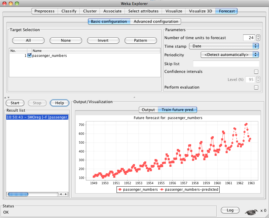
3.1.1 Target selection
At the top left of the basic configuration panel is an area that allows the user to select which target field(s) in the data they wish to forecast. The system can jointly model multiple target fields simultaneously in order to capture dependencies between them. Because of this, modeling several series simultaneously can give different results for each series than modeling them individually. When there is only a single target in the data then the system selects it automatically. In the situation where there are potentially multiple targets the user must select them manually. The screenshot below shows some results on another benchmark data set. In this case the data is monthly sales (in litres per month) of Australian wines. There are six categories of wine in the data, and sales were recorded on a monthly basis from the beginning of 1980 through to the middle of 1995. Forecasting has modeled two series simultaneously: "Fortified" and "Dry-white". 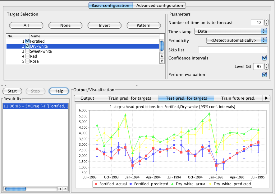
3.1.2 Basic parameters
At the top right of the basic configuration panel is an area with several simple parameters that control the behavior of the forecasting algorithm.
Number of time units
The first, and most important of these, is the Number of time units to forecast text box. This controls how many time steps into the future the forecaster will produce predictions for. The default is set to 1, i.e. the system will make a single 1-step-ahead prediction. For the airline data we set this to 24 (to make monthly predictions into the future for a two year period) and for the wine data we set it to 12 (to make monthly predictions into the future for a one year period). The units correspond to the periodicity of the data (if known). For example, with data recorded on a daily basis the time units are days.
Time stamp
Next is the Time stamp drop-down box. This allows the user to select which, if any, field in the data holds the time stamp. If there is a date field in the data then the system selects this automatically. If there is no date present in the data then the "<Use an artificial time index>" option is selected automatically. The user may select the time stamp manually; and will need to do so if the time stamp is a non-date numeric field (because the system can't distinguish this from a potential target field). The user also has the option of selecting "<None>" from the drop-down box in order to tell the system that no time stamp (artificial or otherwise) is to be used.
Periodicity
Underneath the Time stamp drop-down box is a drop-down box that allows the user to specify the Periodicity of the data. If a date field has been selected as the time stamp, then the system can use heuristics to automatically detect the periodicity - "<Detect automatically>" will be set as the default if the system has found and set a date attribute as the time stamp initially. If the time stamp is not a date, then the user can explicitly tell the system what the periodicity is or select "<Unknown>" if it is not known. Periodicity is used to set reasonable defaults for the creation of lagged variables (covered below in the Advanced Configuration section). In the case where the time stamp is a date, Periodicity is also used to create a default set of fields derived from the date. E.g. for a monthly periodicity, month of the year and quarter fields are automatically created.
Skip list
Below the Periodicity drop-down box is a field that allows the user to specify time periods that should not count as a time stamp increment with respect to the modeling, forecasting and visualization process. For example, consider daily trading data for a given stock. The market is closed for trading over the weekend and on public holidays, so these time periods do not count as an increment and the difference, for example, between market close on Friday and on the following Monday is one time unit (not three). The heuristic used to automatically detect periodicity can't cope with these "holes" in the data, so the user must specify a periodicity to use and supply the time periods that are not to considered as increments in the Skip list text field.
The Skip list field can accept strings such as "weekend", "sat", "tuesday", "mar" and "october", specific dates (with optional formatting string) such as "2011-07-04@yyyy-MM-dd", and integers (that get interpreted differently depending on the specified periodicity). For daily data an integer is interpreted as the day of the year; for hourly data it is the hour of the day and for monthly data it is the month of the year. For specific dates, the system has a default formatting string ("yyyy-MM-dd'T'HH:mm:ss") or the user can specify one to use by suffixing the date with "@<format>". If all dates in the list have the same format, then it only has to be specified once (for the first date present in the list) and then this will become the default format for subsequent dates in the list.
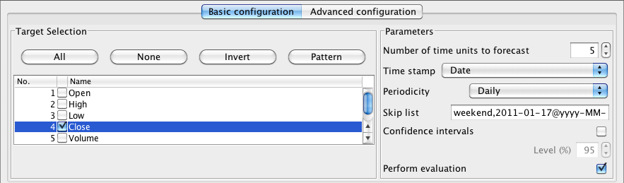
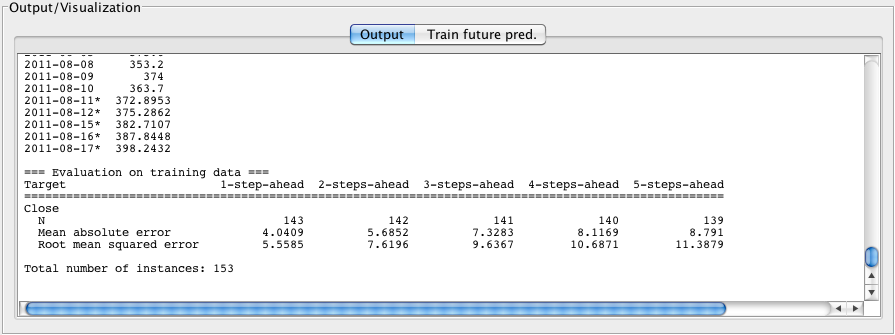
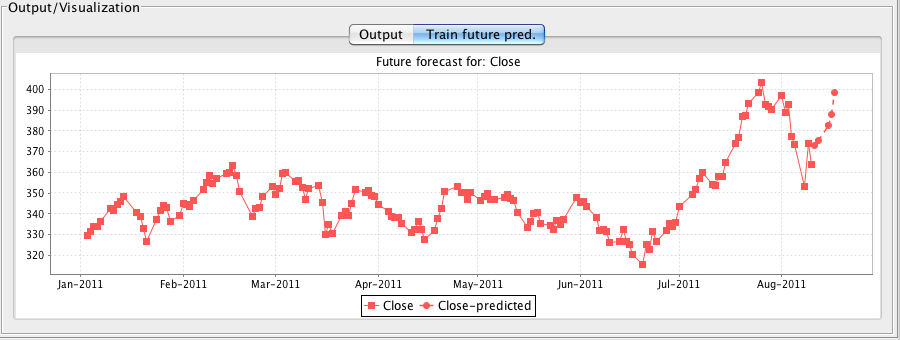
The following screenshots show an example for the "appleStocks2011" data (found in sample-data directory of the package). This file contains daily high, low, opening and closing data for Apple computer stocks from January 3rd to August 10th 2011. The data was take from Yahoo finance (http://finance.yahoo.com/q/hp?s=AAPL&a=00&b=3&c=2011&d=07&e=10&f=2011&g=d). A five day forecast for the daily closing value has been set, a maximum lag of 10 configured (see "Lag creation" in Section 3.2), periodicity set to "Daily" and the following Skip list entries provided in order to cover weekends and public holidays:
weekend, 2011-01-17@yyyy-MM-dd, 2011-02-21, 2011-04-22, 2011-05-30, 2011-07-04
Note that it is important to enter dates for public holidays (and any other dates that do not count as increments) that will occur during the future time period that is being forecasted.
Confidence intervals
Below the Time stamp drop-down box is a check box and text field that the user can opt to have the system compute confidence bounds on the predictions that it makes. The default confidence level is 95%. The system uses predictions made for the known target values in the training data to set the confidence bounds. So, a 95% confidence level means that 95% of the true target values fell within the interval. Note that the confidence intervals are computed for each step-ahead level independently, i.e. all the one-step-ahead predictions on the training data are used to compute the one-step-ahead confidence interval, all the two-step-ahead predictions are used to compute the two-step-ahead interval, and so on.
Perform evaluation
By default, the system is set up to learn the forecasting model and generate a forecast beyond the end of the training data. Selecting the Perform evaluation check box tells the system to perform an evaluation of the forecaster using the training data. That is, once the forecaster has been trained on the data, it is then applied to make a forecast at each time point (in order) by stepping through the data. These predictions are collected and summarized, using various metrics, for each future time step forecasted, i.e. all the one-step-ahead predictions are collected and summarized, all the two-step-ahead predictions are collected and summarized, and so on. This allows the user to see, to a certain degree, how forecasts further out in time compare to those closer in time. The Advanced Configuration panel allows the user to fine tune configuration by selecting which metrics to compute and whether to hold-out some data from the end of the training data as a separate test set.
The following screenshot shows the default evaluation on the Australian wine training data for the "Fortified" and "Dry-white" targets. 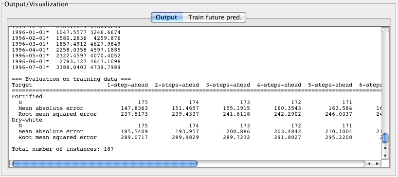
3.1.3 Output
Output generated by settings available from the basic configuration panel includes the training evaluation (shown in the previous screenshot), graphs of forecasted values beyond the end of the training data (as shown in Section 3.1), forecasted values in text form and a textual description of the model learned. There are more options for output available in the advanced configuration panel (discussed in the next section). The next screenshot shows the model learned on the airline data. By default, the time series environment is configured to learn a linear model, that is, a linear support vector machine to be precise. Full control over the underlying model learned and its parameters is available in the advanced configuration panel. 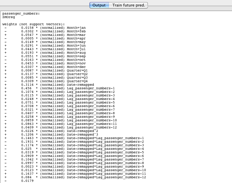
Results of time series analysis are saved into a Result list on the lower left-hand side of the display. An entry in this list is created each time a forecasting analysis is launched by pressing the Start button. All textual output and graphs associated with an analysis run are stored with their respective entry in the list. Also stored in the list is the forecasting model itself. The model can be exported to disk by selecting Save forecasting model from a contextual popup menu that appears when right-clicking on an entry in the list. 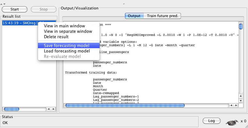
It is important to realize that, when saving a model, the model that gets saved is the one that is built on the training data corresponding to that entry in the history list. If performing an evaluation where some of the data is held out as a separate test set (see below in Section 3.2) then the model saved has only been trained on part of the available data. It is a good idea to turn off hold-out evaluation and construct a model on all the available data before saving the model.
3.2 Advanced Configuration
The advanced configuration panel gives the user full control over a number of aspects of the forecasting analysis. These include the choice of underlying model and parameters, creation of lagged variables, creation of variables derived from a date time stamp, specification of "overlay" data, evaluation options and control over what output is created. Each of these has a dedicated sub-panel in the advanced configuration and is discussed in the following sections.
3.2.1 Base learner
The Base learner panel provides control over which Weka learning algorithm is used to model the time series. It also allows the user to configure parameters specific to the learning algorithm selected. 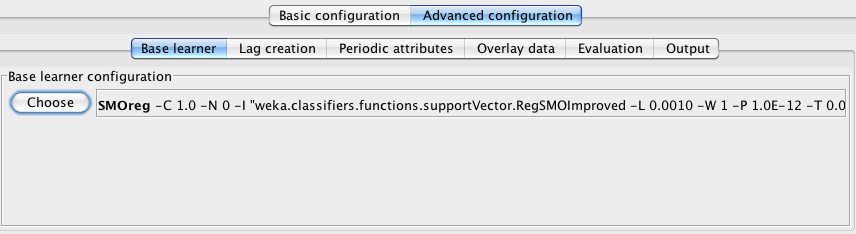
By default, the analysis environment is configured to use a linear support vector machine for regression (Weka's SMOreg). This can easily be changed by pressing the Choose button and selecting another algorithm capable of predicting a numeric quantity. 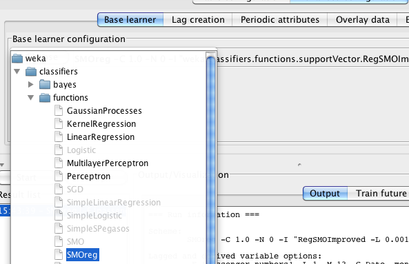
Adjusting the individual parameters of the selected learning algorithm can be accomplished by clicking on the options panel, found immediately to the right of the Choose button. Doing so brings up an options dialog for the learning algorithm. 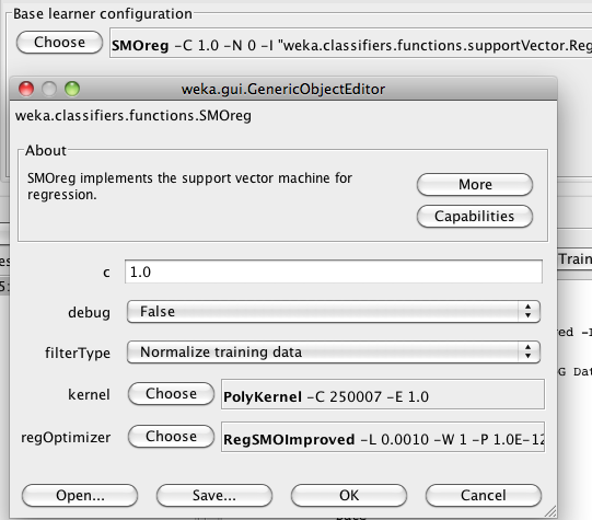
3.2.2 Lag creation
The Lag creation panel allows the user to control and manipulate how lagged variables are created. Lagged variables are the main mechanism by which the relationship between past and current values of a series can be captured by propositional learning algorithms. They create a "window" or "snapshot" over a time period. Essentially, the number of lagged variables created determines the size of the window. The basic configuration panel uses the Periodicity setting to set reasonable default values for the number of lagged variables (and hence the window size) created. For example, if you had monthly sales data then including lags up to 12 time steps into the past would make sense; for hourly data, you might want lags up to 24 time steps or perhaps 12.
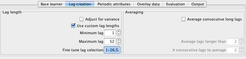
The left-hand side of the lag creation panel has an area called lag length that contains controls for setting and fine-tuning lag lengths. At the top of this area there is a Adjust for variance check box which allows the user to opt to have the system compensate for variance in the data. It does this by taking the log of each target before creating lagged variables and building the model. This can be useful if the variance (how much the data jumps around) increases or decreases over the course of time. Adjusting for variance may, or may not, improve performance. It is best to experiment and see if it helps for the data/parameter selection combination at hand. Below the adjust for variance check box is a Use custom lag lengths check box. This allows the user to alter the default lag lengths that are set by the basic configuration panel. Note that the numbers shown for the lengths are not necessarily the defaults that will be used. If the user has selected "<Detect automatically>" in the periodicity drop-down box on the basic configuration panel then the actual default lag lengths get set when the data gets analysed at run time. The Minimum lag text field allows the user to specify the minimum previous time step to create a lagged field for - e.g. a value of 1 means that a lagged variable will be created that holds target values at time - 1. The Maximum lag text field specifies the maximum previous time step to create a lagged variable for - e.g. a value of 12 means that a lagged variable will be created that holds target values at time - 12. All time periods between the minimum and maximum lag will be turned into lagged variables. It is possible to fine tune the creation of variables within the minimum and maximum by entering a range in the Fine tune lag selection text field. In the screenshot below we have weekly data so have opted to set minimum and maximum lags to 1 and 52 respectively. Within this we have opted to only create lags 1-26 and 52.
On the right-hand side of the lag creation panel is an area called Averaging. Selecting the Average consecutive long lags check box enables the number of lagged variables to be reduced by averaging the values of several consecutive (in time) variables. This can be useful when you want to have a wide window over the data but perhaps don't have a lot of historical data points. A rule of thumb states that you should have at least 10 times as many rows as fields (there are exceptions to this depending on the learning algorithm - e.g. support vector machines can work very will in cases where there are many more fields than rows). Averaging a number of consecutive lagged variables into a single field reduces the number of input fields with probably minimal loss of information (for long lags at least). The Average lags longer than text field allows the user to specify when the averaging process will begin. For example, in the screenshot above this is set to 2, meaning that the time - 1 and time - 2 lagged variables will be left untouched while time - 3 and higher will be replaced with averages. The # consecutive lags to average controls how many lagged variables will be part of each averaged group. For example, in the screenshot above this is also set to 2, meaning that time - 3 and time - 4 will be averaged to form a new field; time - 5 and time - 6 will be averaged to form a new field; and so on. Note that only consecutive lagged variable will be averaged, so in the example above, where we have already fine-tuned the lag creation by selecting lags 1-26 and 52, time - 26 would never be averaged with time - 52 because they are not consecutive.
3.2.3 Periodic attributes
The Periodic attributes panel allows the user to customize which date-derived periodic attributes are created. This functionality is only available if the data contains a date time stamp. If the time stamp is a date, then certain defaults (as determined by the Periodicity setting from the basic configuration panel) are automatically set. For example, if the data has a monthly time interval then month of the year and quarter are automatically included as variables in the data. The user can select the customize checkbox in the date-derived periodic creation area to disable, select and create new custom date-derived variables. When the checkbox is selected the user is presented with a set of pre-defined variables as shown in the following screenshot: 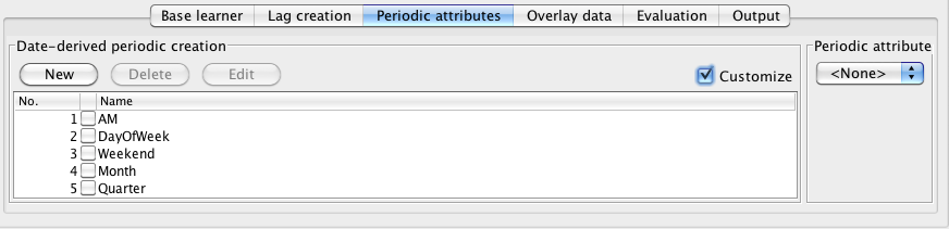
Leaving all of the default variables unselected will result in no date-derived variables being created. Aside from the predefined defaults, it is possible to create custom date-derived variables. A new custom date-derived variable, based on a rule, can be created by pressing the New button. This brings up an editor as shown below: 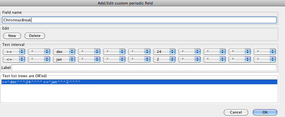
In this example, we have created a custom date-derived variable called "ChistmasBreak" that comprises a single date-based test (shown in the list area at the bottom of the dialog). This variable is boolean and will take on the value 1 when the date lies between December 24th and January 2nd inclusive. Additional tests can be added to allow the rule to evaluate to true for disjoint periods in time.
The Field name text field allows the user to give the new variable a name. Below this are two buttons. The New button adds a new test to the rule and the Delete button deletes the currently selected test from the list at the bottom. Selecting a test in the list copies its values to the drop-down boxes for the upper and lower bounds of the test, as shown in the Test interval area of the screenshot above. Each drop-down box edits one element of a bound. They are (from left to right): comparison operator, year, month of the year, week of the year, week of the month, day of the year, day of the month, day of the week, hour of the day, minute of the hour and second. Tool tips giving the function of each appear when the mouse hovers over each drop-down box. Each drop-down box contains the legal values for that element of the bound. Asterix characters ("*") are "wildcards" and match anything.
Below the Test interval area is a Label text field. This allows a string label to be associated with each test interval in a rule. All the intervals in a rule must have a label, or none of them. Having some intervals with a label and some without will generate an error. If all intervals have a label, then these will be used to set the value of the custom field associated with the rule instead of just 0 or 1. Evaluation of the rule proceeds as a list, i.e. from top to bottom, and the first interval that evaluates to true is the one that is used to set the value of the field. A default label (i.e. one that gets assigned if no other test interval matches) can be set up by using all wildcards for the last test interval in the list. In the case where all intervals have labels, and if there is no "catch-all" default set up, then the value for the custom field will be set to missing if no interval matches. This is different to the case where labels are not used and the field is a binary flag - in this case, the failure to match an interval results in the value of the custom field being set to 0.
3.2.4 Overlay data
The Overlay data panel allows the user to specify fields (if any) that should be considered as "overlay" data. The default is not to use overlay data. By "overlay" data we mean input fields that are to be considered external to the data transformation and closed-loop forecasting processes. That is, data that is not to be forecasted, can't be derived automatically and will be supplied for the future time periods to be forecasted. In the screenshot below, the Australian wine data has been loaded into the system and Fortified has been selected as the target to forecast. By selecting the Use overlay data checkbox, the system shows the remaining fields in the data that have not been selected as either targets or the time stamp. These fields are available for use as overlay data. 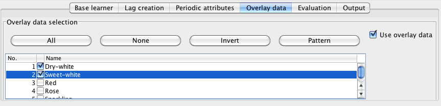
The system will use selected overlay fields as inputs to the model. In this way it is possible for the model to take into account special historical conditions (e.g. stock market crash) and factor in conditions that will occur at known points in the future (e.g. irregular sales promotions that have occurred historically and are planned for the future). Such variables are often referred to as intervention variables in the time series literature.
When executing an analysis that uses overlay data the system may report that it is unable to generate a forecast beyond the end of the data. This is because we don't have values for the overlay fields for the time periods requested, so the model is unable to generate a forecast for the selected target(s). Note that it is possible to evaluate the model on the training data and/or data held-out from the end of the training data because this data does contain values for overlay fields. More information on making forecasts that involve overlay data is given in the documentation on the forecasting plugin step for Pentaho Data Integration.
3.2.5 Evaluation
The Evaluation panel allows the user to select which evaluation metrics they wish to see, and configure whether to evaluate using the training data and/or a set of data held out from the end of the training data. Selecting Perform evaluation in the Basic configuration panel is equivalent to selecting Evaluate on training here. By default, the mean absolute error (MAE) and root mean square error (RMSE) of the predictions are computed. The user can select which metrics to compute in the Metrics area in on the left-hand side of the panel. The available metrics are:
- Mean absolute error (MAE): sum(abs(predicted - actual)) / N
- Mean squared error (MSE): sum((predicted - actual)^2) / N
- Root mean squared error (RMSE): sqrt(sum((predicted - actual)^2) / N)
- Mean absolute percentage error (MAPE): sum(abs((predicted - actual) / actual)) / N
- Direction accuracy (DAC): count(sign(actual_current - actual_previous) == sign(pred_current - pred_previous)) / N
- Relative absolute error (RAE): sum(abs(predicted - actual)) / sum(abs(previous_target - actual))
- Root relative squared error (RRSE): sqrt(sum((predicted - actual)^2) / N) / sqrt(sum(previous_target - actual)^2) / N)
The relative measures give an indication of how the well forecaster's predictions are doing compared to just using the last known target value as the prediction. They are expressed as a percentage, and lower values indicate that the forecasted values are better predictions than just using the last known target value. A score of >=100 indicates that the forecaster is doing no better (or even worse) than predicting the last known target value. Note that the last known target value is relative to the step at which the forecast is being made - e.g. a 12-step-ahead prediction is compared relative to using the target value 12 time steps prior as the prediction (since this is the last "known" actual target value).
The text field to the right of the Evaluate on held out training check box allows the user to select how much of the training data to hold out from the end of the series in order to form an independent test set. The number entered here can either indicate an absolute number of rows, or can be a fraction of the training data (expressed as a number between 0 and 1).
3.2.6 Output
The Output panel provides options that control what textual and graphical output are produced by the system. The panel is split into two sections: Output options and Graphing options. The former controls what textual output appears in the main Output area of the environment, while the latter controls which graphs are generated. 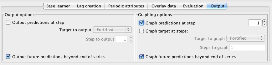
In the Output area of the panel, selecting Output predictions at step causes the system to output the actual and predicted values for a single target at a single step. The error is also output. For example, the 5-step ahead predictions on a hold-out test set for the "Fortified" target in the Australian wine data is shown in the following screenshot. 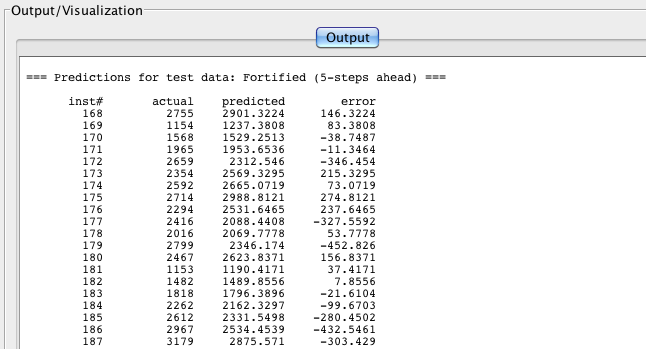
Selecting Output future predictions beyond the end of series will cause the system to output the training data and predicted values (up to the maximum number of time units) beyond the end of the data for all targets predicted by the forecaster. Forecasted values are marked with a "*" to make the boundary between training values and forecasted values clear.
In the Graphing options area of the panel the user can select which graphs are generated by the system. Similar to the textual output, the predictions at a specific step can be graphed by selecting the Graph predictions at step check box. Unlike the textual output, all targets predicted by the forecaster will be graphed. Selecting the Graph target at steps checkbox allows a single target to be graphed at more than one step - e.g. a graph can be generated that shows 1-step-ahead, 2-step-ahead and 5-step ahead predictions for the same target. The Target to graph drop-down box and the Steps to graph text field become active when the Graph target at steps checkbox is selected. The following screenshot shows graphing the the "Fortified" target from the Australian wine data on a hold-out set at steps 1,2,3,6 and 12. 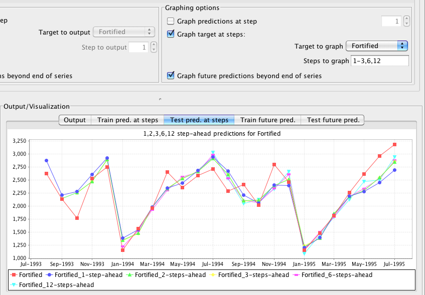
4 Using the API
Here is an example that shows how to build a forecasting model and make a forecast programatically. Javadoc for the time series forecasting package can be found at http://weka.sourceforge.net/doc.packages/timeseriesForecasting/
import java.io.*;

import java.util.List;
import weka.core.Instances;
import weka.classifiers.functions.GaussianProcesses;
import weka.classifiers.evaluation.NumericPrediction;
import weka.classifiers.timeseries.WekaForecaster;
import weka.classifiers.timeseries.core.TSLagMaker;

/**
 * Example of using the time series forecasting API. To compile and
 * run the CLASSPATH will need to contain:
 *
 * weka.jar (from your weka distribution)
 * pdm-timeseriesforecasting-ce-TRUNK-SNAPSHOT.jar (from the time series package)
 * jcommon-1.0.14.jar (from the time series package lib directory)
 * jfreechart-1.0.13.jar (from the time series package lib directory)
 */
public class TimeSeriesExample {

  public static void main(String[] args) {
    try {
      // path to the Australian wine data included with the time series forecasting
      // package
      String pathToWineData = weka.core.WekaPackageManager.PACKAGES_DIR.toString()
        + File.separator + "timeseriesForecasting" + File.separator + "sample-data"
        + File.separator + "wine.arff";

      // load the wine data
      Instances wine = new Instances(new BufferedReader(new FileReader(pathToWineData)));

      // new forecaster
      WekaForecaster forecaster = new WekaForecaster();

      // set the targets we want to forecast. This method calls
      // setFieldsToLag() on the lag maker object for us
      forecaster.setFieldsToForecast("Fortified,Dry-white");

      // default underlying classifier is SMOreg (SVM) - we'll use
      // gaussian processes for regression instead
      forecaster.setBaseForecaster(new GaussianProcesses());

      forecaster.getTSLagMaker().setTimeStampField("Date"); // date time stamp
      forecaster.getTSLagMaker().setMinLag(1);
      forecaster.getTSLagMaker().setMaxLag(12); // monthly data

      // add a month of the year indicator field
      forecaster.getTSLagMaker().setAddMonthOfYear(true);

      // add a quarter of the year indicator field
      forecaster.getTSLagMaker().setAddQuarterOfYear(true);

      // build the model
      forecaster.buildForecaster(wine, System.out);

      // prime the forecaster with enough recent historical data
      // to cover up to the maximum lag. In our case, we could just supply
      // the 12 most recent historical instances, as this covers our maximum
      // lag period
      forecaster.primeForecaster(wine);

      // forecast for 12 units (months) beyond the end of the
      // training data
      List<List<NumericPrediction>> forecast = forecaster.forecast(12, System.out);

      // output the predictions. Outer list is over the steps; inner list is over
      // the targets
      for (int i = 0; i < 12; i++) {
        List<NumericPrediction> predsAtStep = forecast.get(i);
        for (int j = 0; j < 2; j++) {
          NumericPrediction predForTarget = predsAtStep.get(j);
          System.out.print("" + predForTarget.predicted() + " ");
        }
        System.out.println();
      }

      // we can continue to use the trained forecaster for further forecasting
      // by priming with the most recent historical data (as it becomes available).
      // At some stage it becomes prudent to re-build the model using current
      // historical data.

    } catch (Exception ex) {
      ex.printStackTrace();
    }
  }
}
5 Time Series Analysis PDI Spoon Plugin
The time series analysis environment described in the previous sections can also be used within Pentaho Data Integration's Spoon user interface. It appears as a perspective within Spoon and operates in exactly the same way as described above. The only difference is in how data is brought into the time series environment. When running inside of Spoon, data can be sent to the time series environment via a Table Input or Table Output step. Right-clicking on either of these steps brings up a contextual menu; selecting "Forecast" from this menu activates the time series Spoon perspective and loads data from the data base table configured in the Table Input/Output step into the time series environment.